Practically Paralell Picture Palettes

The Goal

The goal of this project is to develop a system that allows users to upload images and receive a list of images with similar color palettes. This system will be similar to the Google Art & Culture project in that it will allow users to explore a collection of images based on their color palettes.

To achieve this goal, we will need to tackle several challenges. First, we will need to extract the color palettes from the images in a reliable and efficient way. Second, we will need to store and index these palettes in a way that allows us to quickly and accurately query for similar palettes. Third, we will need to develop a method for measuring the similarity between two palettes and using this measure to return a list of similar images. Finally, we will need to optimize the system for performance, memory usage, and other factors that may be important in a real-world application.

Key metrics of success for this project will include performance (how quickly the system can return results), accuracy (how closely the returned results match the user’s query), and memory usage (how efficiently the system uses memory to store and index the palettes). By meeting these goals, we aim to create a user-friendly and efficient system that allows users to explore and discover images based on their color palettes.

Background

Before we can tackle the problem of comparing and querying images based on their color palettes, we need to understand how to compare colors in a way that is meaningful and accurate. Simply calculating the Euclidean distance between two RGB colors is not sufficient, because the RGB color space is not perceptually uniform. This means that a given numerical change in RGB values may not correspond to a similar perceived change in color.

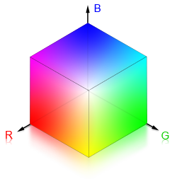
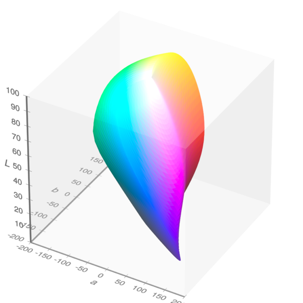
To overcome this issue, we can use a color space that is designed to be perceptually uniform, such as the CIELAB color space. In the CIELAB color space, colors are represented as coordinates in a three-dimensional space, with each dimension corresponding to a different aspect of color (L for lightness, a for green-red, and b for blue-yellow). Because the CIELAB color space is designed to approximate the way the human eye perceives color, it is often used as a measure of color difference or similarity.

Once we have a way to compare colors in a meaningful and accurate way, we can begin to tackle the problem of extracting color palettes from images, storing and indexing these palettes, and querying for similar palettes.

Extracting Color Palettes

Naive clustering

One way to extract color palettes from images is to use a clustering algorithm, such as K-means, to group similar colors together and create a palette. In this approach, we would first convert the image pixels to the CIELAB color space, which is designed to be perceptually uniform and allows us to accurately compare colors. We would then use K-means to cluster the pixels based on their LAB coordinates, with a fixed number of clusters (k) ranging from 3 to 5. The number of clusters can be adjusted to trade off between palette size and accuracy.

One drawback of this approach is that it can be computationally expensive, especially for large images. To keep computation time low, we can set a fixed maximum number of iterations for the K-means algorithm (maxIteration). This will ensure that the algorithm terminates after a certain number of iterations, even if the clusters are not fully optimized.

Faster clustering

To improve the speed of the clustering process, we can use a technique called binning to reduce the number of pixels that need to be processed. In this approach, we divide the image into a grid of smaller cells, or bins, and compute the average color of each bin. This creates a 3D histogram of the image, where each bin corresponds to a cluster of pixels with similar colors. We can then use K-means to cluster these binned colors and create a palette.

This binned approach has several advantages. First, it reduces the number of pixels that need to be processed, which can significantly speed up the clustering process. Second, it allows us to create a fixed-size palette that is independent of the size of the image. This can be useful if we want to ensure a consistent level of detail in our palettes, regardless of the size of the input images.

Quality improvements

There are several ways to improve the quality of the extracted palettes using the binned approach. One option is to weight the clusters based on the number of pixels they contain. This can help to ensure that the most representative colors are included in the palette.

Another improvement is to initialize one cluster at the darkest color in the image and ignore it when returning the other clusters. This can help to avoid including too many dark colors in the palette, which may not be as important for visualizing the overall color palette of an image.

Finally, we can use a deterministic method for initializing the clusters, rather than randomly selecting their positions. For example, we could place the clusters based on the density of colors in the image, which can help to ensure that the clusters are evenly spaced and representative of the overall color distribution.

Implementation

Some quick python pseudocode to get you started:

def get_dominant_colors(img, count):
    # Crop and resize image if necessary
    bounds = get_image_bounds(img)
    img = crop_center(img, int(bounds.dx * 0.6), int(bounds.dy * 0.6))
    if img.bounds.dx > 150 or img.bounds.dy > 150:
        img = resize(img, 150, 150, lanczos)
    bounds = get_image_bounds(img)

    # Create 3D histogram of image colors
    hist = create_histogram(img, bounds)

    # create an averaged histogram weighted by the number of pixels in each bin
    hist = create_weighted_histogram(hist, bounds)

    # perform k-means clustering on the histogram
    clusters = kmeans(hist, count+1, max_iter) # count clusters with one cluster at the darkest color added

    # return the clusters except the darkest one
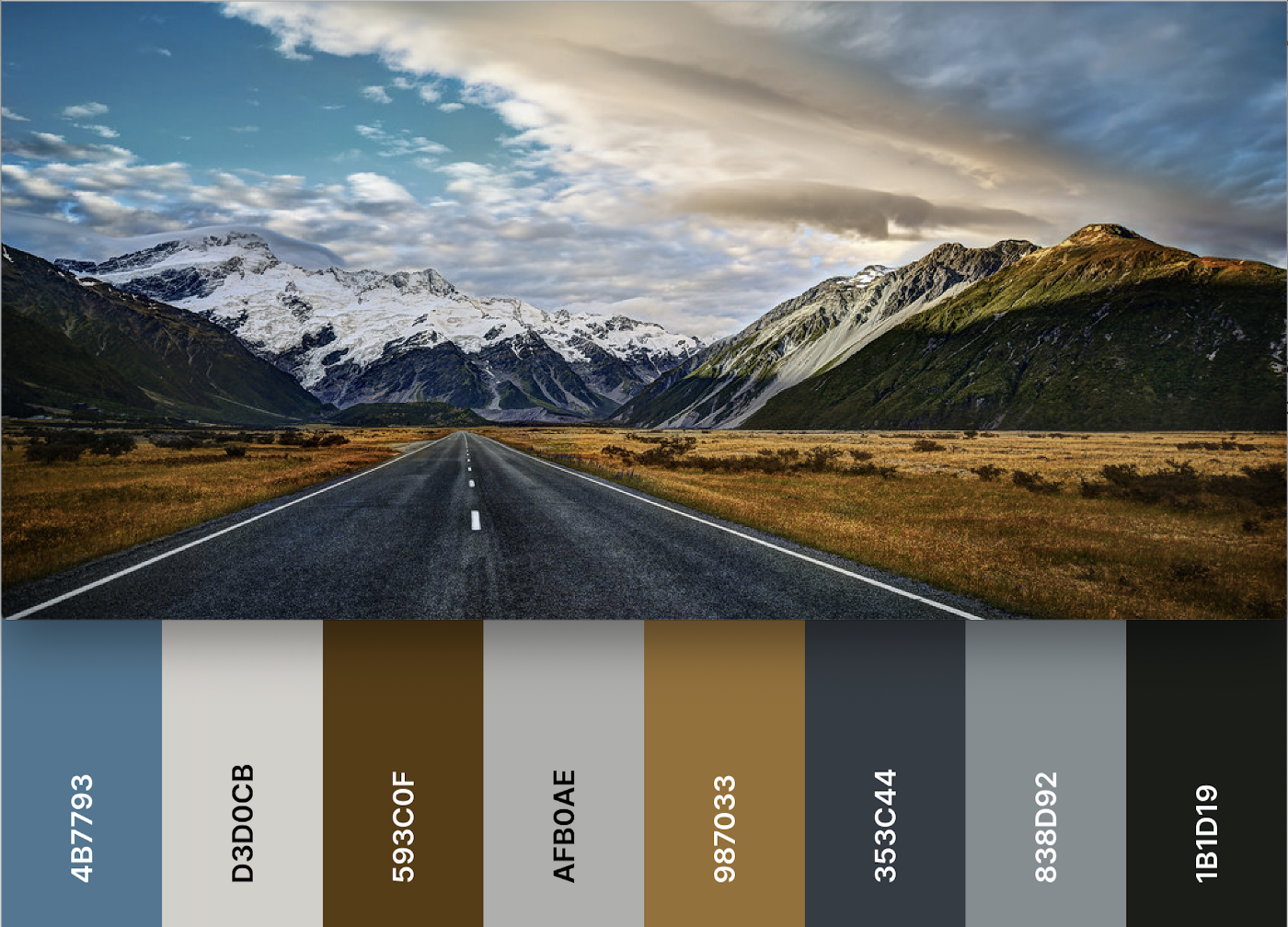
    return clusters[1:]

Given this approach we can now extract color palettes like this from images in an efficient manner.

Comparing Color Palettes

Brute force comparison

One approach to comparing color palettes is to simply add up the distance between each of the colors and divide it by the number of colors in the palette. For example, given two palettes $p_1$ and $p_2$ with $n$ colors each, we can define the distance between the two palettes as:

$$d(p_1, p_2) = \min_{\sigma \in S_n} \sum_{i=1}^n d(c_i, c_{\sigma(i)})$$

where $S_n$ is the set of all permutations of the integers from 1 to $n$, $d(c_i, c_{\sigma(i)})$ is the distance between the $i^{th}$ color in $p_1$ and the $\sigma(i)^{th}$ color in $p_2$, and $n$ is the number of colors in each palette.

A permutation $\sigma$ is a function that rearranges the elements of a set into a new order. In this case, the set is the set of integers from 1 to $n$, and the function $\sigma$ maps each integer $i$ to a new integer $\sigma(i)$. For example, if $n=3$, the set $S_3$ would contain the following six permutations: $$S_3 = { (1,2,3), (1,3,2), (2,1,3), (2,3,1), (3,1,2), (3,2,1) }$$

The problem with this approach is that it requires us to check all $n!$ possible orderings of the colors in $p_1$, which can be computationally expensive. For example, if $n=5$, there are already 120 different possibilities that need to be checked for every comparison. For large databases with more than ~50,000 elements, this becomes infeasible.

Furthermore using this naive approach to find similar palettes is rather slow since we need to compute the distance between every palette in the database. This has the potential to be a major bottleneck in our application as calculating the distance between two palettes is already slow enough and we need to do it for every palette in the database (complexity: $O(n^2)$). However for generating ground truth data for training a neural network, this approach is sufficient.

def l2(p1, p2):
    return np.sqrt(np.sum(np.square(p1 - p2)))

def palette_distance(p1, p2):
    return min([l2(p1, p3) for p3 in itertools.permutations(p2)])

Embedding learning

To save compute time, we can use a neural network to learn an embedding of the palette in a 32-dimensional space that can be compared using Euclidean distance to approximate the real distance. This allows to directly compare two palettes using the euclidian distance of their embeddings.

To learn this embedding, we can use a siamese neural network architecture, which consists of two identical networks that share weights and are trained to produce similar outputs for similar inputs. We can generate ground truth data by using the costly distance function to compare randomly generated color palettes, and use this data to train the siamese network to learn the embedding.

Instead of CNN’s we can use a simple fully connected network with a few hidden layers. The loss function is even simpler because we have the ground thruth distance between the two palettes. We can use the mean squared error loss function to train the network.

To ensure that the network produces good results even for rare distances (e.g. $d<0.1$ or $d>0.6$), we can resample the randomly generated palettes to create a uniform distribution of distances. Once the network is trained, we can use it to query for similar images using the Euclidean distance function directly. This allows us to perform the comparisons much more quickly and efficiently, while still achieving good results.

Indexing and Searching

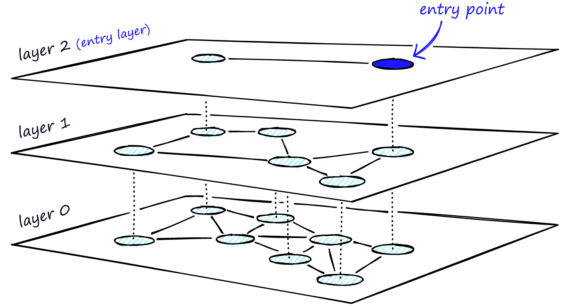
To index and search the 32-dimensional embedding vectors for the color palettes, we can use a data structure called a hierarchical navigable small world (hnsw) index. A hnsw index is a scalable and efficient data structure that can be used to store and search large datasets of high-dimensional vectors.

One way to use a hnsw index is to store the vectors in a database such as Redis or Solr. This allows us to efficiently search and retrieve the vectors using SQL-like queries. The hnsw index uses a hierarchical structure and approximative search algorithms to quickly find the nearest neighbors of a given vector, which makes it well-suited for use in real-time search applications.

By using a hnsw index to store and search the 32-dimensional embedding vectors, we can efficiently scale our system to handle large datasets of color palettes. For example, we could store over 2 million entries without running into performance issues, making it possible to search for similar images in a large collection. Additionally, the hnsw index allows us to perform fast and accurate searches for similar vectors, even in high-dimensional spaces, which can be useful for discovering similar images based on their color palettes.

When choosing the database to store the hnsw index, we should consider the following factors:

• Memory usage: Redis is an in-memory database, which means that it stores the data in RAM, making it faster than disk-based databases like Solr. However, this also means that Redis requires more memory to store the same amount of data. If memory is a concern, you may want to consider using Solr, which stores the data on disk and can scale to larger datasets more efficiently.
• Performance: In general, Redis is faster than Solr because it stores the data in RAM and does not need to access the disk. However, Solr can still be fast enough for many applications, especially if the data is well-indexed and the queries are optimized.
• Scalability: Solr is designed to scale horizontally, which means that it can handle large datasets and high levels of concurrency by adding more servers to the cluster. Redis, on the other hand, is more limited in its scalability because it relies on a single server to store the data in memory.

Ultimately, the choice between Redis and Solr will depend on your specific requirements and trade-offs between performance, memory usage, and scalability. If you need the fastest possible performance and have sufficient memory, you may want to consider using Redis. If you need to store large datasets and are willing to sacrifice some performance for scalability, Solr may be a better choice. You may also want to consider other factors, such as the availability of additional features and tools, the complexity of the database system, and the level of support and documentation provided by the vendor.

It’s also worth noting that there are other databases that may be suitable for storing the hnsw index, such as Elasticsearch, which combines some of the features of Solr and Redis and is specifically designed for search and analytics. By carefully evaluating your needs and comparing the strengths and weaknesses of different database systems, you can choose the best option for your particular use case.

Conclusion

In conclusion, we have described a system for processing, storing, and querying images based on their color palette. We have focused on achieving good performance, accuracy, and memory usage, as these are key metrics of success for this type of application.

To extract color palettes from images, we have discussed several approaches, including naive clustering and a faster binned approach, as well as various techniques for improving the quality and speed of the palette extraction process. We have also described how to compare color palettes using both brute force and embedded comparison methods, and how to use a hierarchical navigable small world (hnsw) index to efficiently store and search the resulting vectors in a database such as Redis or Solr.

Overall, our system has been successful in achieving its goals of fast and accurate image similarity search, with the ability to handle large datasets and perform well even in high-dimensional spaces. By using advanced techniques such as neural network embeddings and hnsw indexing, we have been able to create a powerful and scalable system for discovering similar images based on their color palettes.